Factorial

$n$	$n!$
0	1
1	1
2	2
3	6
4	24
5	120
6	720
7	5040
8	40320
9	362880
10	3628800

In mathematics, the factorial is the meromorphic function with fast growth along the real axis; for non-negative integer values of the argument, this function has integer values. Frequently, the postfix notation $n!$ is used for the factorial of number $n$. For integer $n$, the $n!$ gives the number of ways in which n labelled objects (for example the numbers from 1 to n) can be arranged in order. These are the permutations of the set of objects. In some programming languages, both n! and factorial(n) , or Factorial(n), are recognized as the factorial of the number $n$.

Integer values of the argument

For integer values of the argument, the factorial can be defined by a recurrence relation. If n labelled objects have to be assigned to n places, then the n-th object can be placed in one of n places: the remaining n-1 objects then have to be placed in the remaining n-1 places, and this is the same problem for the smaller set. So we have

$n!=n\cdot (n-1)!\,$

and it follows that

$n!=n\cdot (n-1)\cdots 2\cdot 1,\,$

which we could derive directly by noting that the first element can be placed in n ways, the second in n-1 ways, and so on until the last element can be placed in only one remaining way.

Since zero objects can be arranged in just one way ("do nothing") it is conventional to put 0! = 1.

The factorial function is found in many combinatorial counting problems. For example, the binomial coefficients, which count the number of subsets size r drawn from a set of n objects, can be expressed as

${\binom {n}{r}}={\frac {n!}{r!(n-r)!}}.$

The factorial function can be extended to arguments other than positive integers: this gives rise to the Gamma function.

Definitions

For complex values of the argument, the combinatoric definition above should be extended.

Implicit definition

The factorial can be defined as unique meromorphic function $F$, satisfying relations

$F(z+1)=(z+1)F(z)$

$F(0)=1$

for all complex $z$ except negative integer values. The uniqueness of function $F$, satisfying these equations, follows from the Wielandt's theorem . Historically, the deduction refers to the Gamma function, but the application to the factorial is straightforward.

Definition through the integral

Usually, the integral representation is used as definition. For $\Re (z)>-1$, define

$z!=\int _{0}^{\infty }t^{z}\exp(-t)\mathrm {d} t$

Such definition is similar to that of the Gamma function, and leads to the relation

$z!=\Gamma (z+1)$

for all complex $z$ except the negative integer values.

The definition above agrees with the combinatoric definition for integer values of the argument; at integer $z$, the integral can be expressed in terms of the elementary functions.

Extension of integral definition

$f=z!$ in the complex $z$-plane.

The definition through the integral can be extended to the whole complex plane, using relation

$z!=(z+1)!/(z+1)$

for the cases $\Re (z)<-1$, assuming that $z$ is not negative integer. Also, the symmetry formula takes place for the non-integer values of $z$,

$z!(-z)!={\frac {\pi z}{\sin(\pi z)}}$

The similar formula of symmetry holds however, for the Gamma function. From this expression, it follows that ${\frac {1}{z!(-z)!}}$ is entire function of $z$. Also, this symmetry gives the simple way to express $(1/2)!={\sqrt {\pi }}/2$, and, therefore, factorial of half-integer numbers.

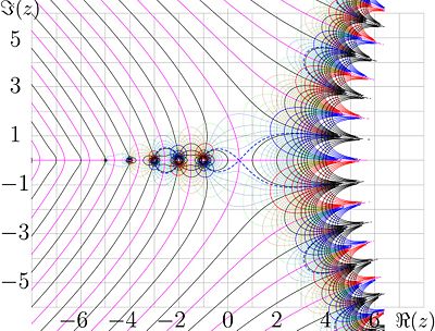
In the figure, lines of constant $u=\Re (z!)$ and lines of constant $v=\Im (z!)$ are shown.
The levels u = − 24, − 20, − 16, − 12, − 8, − 7, − 6, − 5, − 4, − 3, − 2, − 1,0,1,2,3,4,5,6,7,8,12,16,20,24 are drown with thick black lines.
Some of intermediate levels u = const are shown with thin blue lines for positive values and with thin red lines for negative values.
The levels v = − 24, − 20, − 16, − 12, − 8, − 7, − 6, − 5, − 4, − 3, − 2, − 1 are shown with thick red lines.
The level v = 0 is shown with thick pink lines.
The levels v = 1,2,3,4,5,6,7,8,12,16,20,24 are drown with thick blue lines. some of intermediate levels v = const are shown with thin green lines.
The dashed blue line shows the level $u=\mu _{0}$ and corresponds to the value $\mu _{0}=(x_{0})!\approx 0.85$ of the principal local minimum $x_{0}\approx 0.45$ of the factorial of the real argument.
The dashed red line shows the level and corresponds to the similar value of the negative local extremum of the factorial of the real argument.
Due to the fast growth of the function, in the right hand side of the figure, the density of the levels exceeds the ability of the plotter to draw them; so, this part is left empty.

Factorial of the real argument

$\mathrm {factorial} (x)=x!$; the inverse function, id est, $\mathrm {factorial} ^{-1}(x)$, and $\mathrm {factorial} (x)^{-1}$ versus real $x$.

The definition above was elaborated for factorial of complex argument. In particular, it can be used to evaluate the factorial of the real argument. In the figure at right, the $\mathrm {factorial} (x)=x!$ is plotted versus real $x$ with red line. The function has simple poluses at negative integer $x$.

At $x\rightarrow -1+o$, the $x!\rightarrow +\infty$.

The local minimum

The factorial has local minimum at

$x=\nu _{0}\approx$0.461632144968362341262659542325721328468196204

marked in the picture with pink vertical line; at this point, the derivative of the factorial is zero:

$\mathrm {factorial} ^{\prime }(\nu _{0})=0$

The value of factorial in this point

$\mu _{0}=\nu _{0}!=\mathrm {factorial(\nu _{0})} \approx$0.88560319441088870027881590058258873320795153367

The Tailor expansion of $z!$ at the point $z=\nu _{0}$ can be written as follows:

$z!=\mu _{0}+\sum _{n=2}^{N-1}c_{n}(z-\nu _{0})^{n}+{\mathcal {O}}(z-\nu _{0})^{N}~$ .

The coefficients of this expansion are copypasted in the table below:

$n$	approximation of $c_{n}$
2	0.428486815855585429730209907810650582960483696962
3	-0.130704158939785761928008749242671025181542078103
4	0.160890753325112844190519489594363387594505844657
5	-0.092277030213334350126864106458600575084335085690

This expansion can be used for the precise evaluation of the inverse function of factorial (arcfactorial) in vicinity of the branchpoint.

Other local extremums are at negative values of the argument; one of them in shown in the figure above.

The Taylor expansion

The Taylor expansion of $z!$ at $z=0$, or the MacLaurin expansion, has the form $z!=\sum _{n=0}^{N-1}g_{n}z^{n}+{\mathcal {O}}(z^{N})~$ . The first coefficients of this expansion are copypasted in the table below:

$n$	$g_{n}$	approximation of $g_{n}$
0	$1$	$1.000000000000000000000000000000000000000000000000000000000000$
1	$~-\gamma ~$	$-0.577215664901532860606512090082402431042159335939923598805767$
2	${\frac {\pi ^{2}}{12}}+{\frac {\gamma ^{2}}{2}}$	$0.989055995327972555395395651500634707939183520728214090443192$
3	$-{\frac {\zeta (3)}{3}}-{\frac {\pi ^{2}\gamma }{12}}+{\frac {\gamma ^{3}}{6}}$	$-0.907479076080886289016560167356275114928611449072563760941328$
4	${\frac {\pi ^{4}}{160}}+{\frac {\zeta (3)}{3}}-{\frac {\pi ^{2}\gamma ^{2}}{12}}+{\frac {\gamma ^{4}}{24}}$	$0.981728086834400187336380294021850850360573679723465415404953$

Here, $\gamma$ is the Euler constant and $\zeta$ is the Riemann function. The Computer algebra systems such as Maple and Mathematica can generate many terms of this expansion. The radius of convergence of the Taylor series is unity, and the coefficient $g_{n}$ does not decay as $n$ increases. However, due to the relation $z!=z\cdot \mathrm {factorial} (z)$, for any real value of argument of factorial, the expansion above can be used for the precise evaluation of factorial of the real argument, running the approximation above for an argument with modulus not larger than half. Also, the expansion at the half-integer values can be used: $z!=\sum _{n=0}^{N-1}h_{n}~\left(z-{\frac {1}{2}}\right)^{n}+{\mathcal {O}}\left(\left(z-{\frac {1}{2}}\right)^{N}\right)~$ . The first coefficients of this expansion are copypasted in the table below:

$n$	$h_{n}$	approximation of $g_{n}$
0	${\frac {\sqrt {\pi }}{2}}$	$0.886226925452758013649083741670572591398774728061193564106905$
1	${\frac {-{\sqrt {\pi }}}{2}}(\gamma +\log(4)-2)$	$0.0323383974488850138288698842689703077813347888705070206366386$
2	${\frac {\pi ^{5/2}}{8}}+{\sqrt {\pi }}\gamma -{\sqrt {\pi }}\log(4)+{\frac {\gamma ^{2}{\sqrt {\pi }}}{4}}+{\sqrt {\pi }}\log(2)^{2}$	$0.414813453688301168230037623111356342848909963370422367977736$
3	long expression	$-0.107294804564772211687541956389709662054575923821298300938631$
4	even longer expression	$0.144645359044621543038332210253884524070026861530981428414028$

The Taylor series of $z!$ developed at $z=1/2$, converges for all $z$ such that $|z-1/2|<3/2$.

In order to boost the approximation of factorial for real values of the argument, and, especially, for the evaluation for complex values, and the evaluation of the inverse function, the expansions for $\log(z!)$ and $1/z!$ are used instead of the direct Taylor expansions above.

Halving of the imaginary part of the argument

While neither $z$ nor $(z+1)/2$ is negative integer, the argument of factorial can be dropped with the identity

$\mathrm {Factorial} (z)~=~{\frac {2^{z}}{\sqrt {\pi }}}~\mathrm {Factorial} \!\left({\frac {z}{2}}\right)\cdot \mathrm {Factorial} \!\left({\frac {z\!-\!1}{2}}\right)$

This may be useful to drop with factor 1/2 the imaginary part of the argument (for example, to apply the Taylor expansion above for the evaluation), but the function has to be evaluated twice.

Related functions

(CC) Image: Dmitrii Kouznetsov
ArcFactorial in the complex plane.

In the plot of factorial of the real argument, the two other functions are plotted, $\mathrm {ArcFactorial} (x)=\mathrm {factorial} ^{-1}(x)$ and $\mathrm {factorial} (x)^{-1}$. These functions can be useful for the generalization of the factorial and for its evaluation.

Inverse function

$z$	ArcFactorial$(z)$
$\mu _{0}$	0.46163214496836234126265954233
${\frac {\sqrt {\pi }}{2}}$	0.50000000000000000000000000000
1	1.00000000000000000000000000000
2	2.00000000000000000000000000000
3	2.40586998630956692469992921838
4	2.66403279720644615568638939436
5	2.85235545803172783164299808684
6	3.00000000000000000000000000000

Inverse function of factorial can be defined with equation

$(\mathrm {ArcFactorial} (z))!=z$

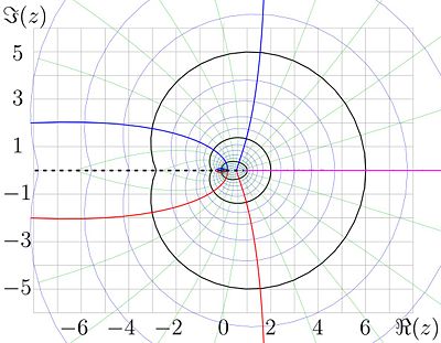
and condition that ArcFactorial is holomorphic in the comlex plane with cut along the part of the real axis, that begins at the minimum value of the factorial of the positive argument, and extends to $-\infty$. This function is shown with lines of constant real part $u=\Re (\mathrm {ArcFactorial} (z))$ and lines of constant imaginary part $v=\Im (\mathrm {ArcFactorial} (z))$.

Levels $u=1,2,3$ are shown with thick black curves.
Levels $u=0.2,0.4,0.6,0.8,1.2,1.4,1.6,1.8,2.2,2.4,2.6,2.8,3.2,3.4,3.6$ are shown with thin blue curves.
Levels $v=1,2,3$ are shown with thick blue curves.
Level $v=0$ is shown with thick pink line.
Levels $v=-1,-2,-3$ are shown with thick red curves.
The intermediate levels of constant $v$ are shown with thin dark green curves. The ArcFactorial has the branch point $\mu _{0}\approx 0.85$; the cut of the range of holomorphism is shown with black dashed line.

ArcFactorial for some real values of the argument is approximated in the table at right.

$n$	approximation for $d_{n}$
1	1.43764234228440800
2	0.315227181071631549
3	-0.0256407066268564423
4	0.00492170392390056555

In vicinity of the branchpoint $z=\mu _{0}$, the ArcFactorial can be expanded as follows:

$\mathrm {ArcFactorial} (z)=\nu _{0}+\sum _{n=1}^{N-1}d_{n}\cdot {\Big (}\log(z/\mu _{0}){\Big )}^{n/2}$

The approximations for the first coefficients of this expansion are copypasted in the table at right. About of 30 terms in this expansion are sufficient to plot the distribution of the real and the imaginary parts of ArcFactorial in the figure above.

Function $f(z)=1/z!$

(CC) Image: Dmitrii Kouznetsov
$f(z)={\frac {1}{z!}}$ in the complex $z$-plane.

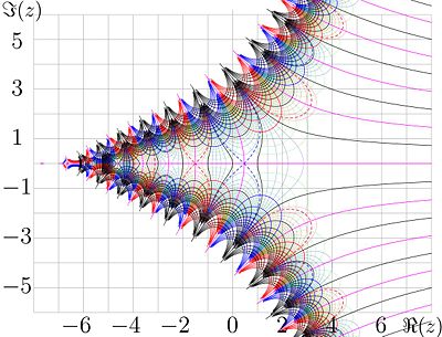
The inverse function of factorial, id est, $\mathrm {ArcFactorial} (z)=\mathrm {Factorial} ^{-1}(z)$ from the previous section, should not be confused with $f(z)={\frac {1}{z!}}=\mathrm {Factorial} (z)^{-1}={\frac {1}{\mathrm {Factorial} (z)}}$ shown in the figure at right. The lines of constant $u=\Re (f(z))$ and the lines of constant $v=\Im (f(z))$ are drawn.
The levels $u=-24,-20,-16,-12,-8,-7..7,8,12,16,20,24$ are shown with thick black lines.
The levels $v=-24,-20,-16,-12,-8,-7...7,-1$ are shown with thick red lines.
The level $v=0$ is shown with thick pink line.
The levels $v=1,2,...7,8,12,16,20,24$ are shown with thick blue lines.
Some of intermediate elvels $u=$const are shown with thin red lines for negative values and thin blue lines for the positive values.
Some of intermediate elvels $v=$const are shown with thin green lines.
The blue dashed curves represent the level $u=1/\mu _{0}$ and correspond to the positive local maximum of the inverse function of the real argument.
The red dashed curves represent the level $u=1/\mu _{1}$, which corresponds to the first negative local maximum of the factorial of the real argument; $\mathrm {factorial} ^{\prime }(\nu _{1})=0$; $\mathrm {factorial} (\nu _{1})=\mu _{1}$.

In the upper-left hand side of the figure, and at the lower-left hand side of the figure, the density of levels exceeds the ability of the ploter to draw them, and these parts are left empty.

$f(z)={\frac {1}{z!}}$ is entire function, that grows in the left hand side of the complex plane and quickly decays to zero along the real axis.

Logfactorial

Template:CC-Image
LogFactorial at the complex plane.

For the approximation of factorial, if can be represented in the form

$z!=\exp(\mathrm {LogFactorial} (z))$

Plof of LogFactorial

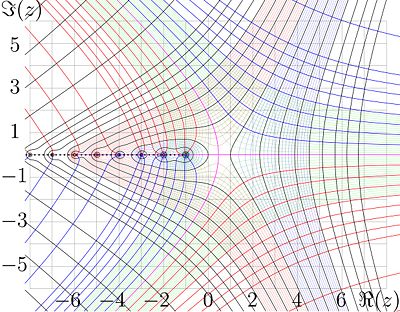
Function LogFactorial is shown in figure with lines of constant real part and lines of constant imaginary part. Levels of constant $u=\Re (\mathrm {LogFactorial} (z))$ and Levels of constant $v=\Im (\mathrm {LogFactorial} (z))$ are drawn with solid lines:
Levels $u=-24,-20,-16,-12,-8,-7,-6,-5,-4,-3,-2,-1,0,1,2,3,4,5,6,7,8,12,16,20,24$ are shown with thick black curves.
Levels $u=-3.8,-3.6,-3.4,-3.2-2.8,-2.6,-2.4,-2.2-1.8,-1.6,-1.4,-1.2-0.8,-0.6,-0.4,-0.2$ are shown with thin red curves.
Levels $u=0.2,0.4,0.6,0.81.2,1.4,1.6,1.82.2,2.4,1.6,2.83.2,3.4,3.6,3.8$ are shown with thin blue curves.
Levels $v=-24,-20,-16,-12,-8,-7,-6,-5,-4,-3,-2,-1$ are shown with thick red curves.
Level $v=0$ is shown with thick pink line.
Levels $v=1,2,3,4,5,6,7,8,12,16,20,24$ are shown with thick blue lines.
Levels $v=-3.8,-3.6,-3.4,-3.2-2.8,-2.6,-2.4,-2.2-1.8,-1.6,-1.4,-1.2-0.8,-0.6,-0.4,-0.20.2,0.4,0.6,0.81.2,1.4,1.6,1.82.2,2.4,1.6,2.83.2,3.4,3.6,3.8$ are shown with thin green curves.
The cut of range of holomorphism is shown with black dashed line.

Function LogFactorial has singularities at the same points, as the factorial, id est, at negative integer values of the argument.

Approximation of LogFactorial at large values of the argument

$n$	$a_{n}$	approximation of $a_{n}$
0	1 / 12	0.083333333333333333
1	1 / 30	0.033333333333333333
2	53 / 210	0.252380952380952381
3	195 / 371	0.525606469002695418

Far from the negative part of the real axis, the function LogFactorial can be approximated through the continual fraction $p$:

$\mathrm {LogFactorial} (z)=p(z)+\log(2\pi )/2-z+(z+1/2)~\log(z)$

$p(z)={\frac {a_{0}}{z+{\frac {a_{1}}{z+{\frac {a_{2}}{z+{\frac {a_{3}}{z+..}}}}}}}}$

The coefficients $a$ and their approximate evaluations are copypasted in the table at right.

In vicinity of the real axis, while the modulus of the imaginary part of LogFactorial does not exceed $\pi$, the LogFactorial can be interpreted as logarithm of factorial, id est,

$\mathrm {LogFactorial} (z)=\log(z!)$

In particular, this relation is valid for positive real values of $z$.

For all $z$ except negative integers, $z!=\exp \!{\Big (}\mathrm {LogFactorial} (z){\Big )}$

However, the LogFactorial has singularities at negative integer valies of the argument.

Stirling formula

Historically, one of the first approximations of the factorial with elementary functions was the Stirling formula below. For large n there is an approximation due to Scottish mathematician James Stirling

$n!\approx {\sqrt {2\pi }}n^{n+1/2}e^{-n}.\,$

This formula can be obtained from the approximation for LogFactorial above, just replacing $p(z)$ to zero.

References

• Ronald L. Graham; Donald E. Knuth, Oren Patashnik (1989). Concrete Mathematics. Addison Wesley, 111,332. ISBN 0-201-14236-8. 

• http://tori.ils.uec.ac.jp/TORI/index.php/Factorial

References

- ↑ Wielandt's theorem online: http://www.math.ku.dk/~henrikp/specialtopic2000/node7.html
- ↑ Reinhold Remmert The American Mathematical Monthly, Vol. 103, No. 3 (Mar., 1996), pp. 214-220, http://www.jstor.org/pss/2975370